Sampling And Normal Distribution Answers

Chapter 6 Sampling Distributions

A statistic, such as the sample hateful or the sample standard deviation, is a number computed from a sample. Since a sample is random, every statistic is a random variable: it varies from sample to sample in a fashion that cannot exist predicted with certainty. Equally a random variable it has a mean, a standard deviation, and a probability distribution. The probability distribution of a statistic is called its sampling distributionThe probability distribution of a sample statistic when the statistic is viewed equally a random variable. . Typically sample statistics are not ends in themselves, but are computed in order to estimate the corresponding population parameters, equally illustrated in the m motion picture of statistics presented in Figure ane.i "The Grand Picture of Statistics" in Chapter 1 "Introduction".

This chapter introduces the concepts of the hateful, the standard deviation, and the sampling distribution of a sample statistic, with an emphasis on the sample mean $\stackrel{-}{\mathit{x}}.$

6.ane The Mean and Standard Departure of the Sample Mean

Learning Objectives

1. To go familiar with the concept of the probability distribution of the sample mean.
2. To empathise the meaning of the formulas for the hateful and standard deviation of the sample mean.

Suppose we wish to estimate the mean μ of a population. In actual exercise nosotros would typically accept just one sample. Imagine however that nosotros take sample afterward sample, all of the same size north, and compute the sample mean $\stackrel{-}{\mathit{ten}}$ of each one. We will probable get a different value of $\stackrel{-}{\mathit{x}}$ each time. The sample mean $\stackrel{-}{\mathit{10}}$ is a random variable: it varies from sample to sample in a way that cannot be predicted with certainty. We will write $\stackrel{-}{\mathit{X}}$ when the sample mean is idea of equally a random variable, and write $\stackrel{-}{\mathit{x}}$ for the values that information technology takes. The random variable $\stackrel{-}{\mathit{X}}$ has a hatefulThe number about which ways computed from samples of the same size eye. , denoted ${\mathit{\mu }}_{\stackrel{-}{\mathit{X}}}$ , and a standard deviationA measure of the variability of means computed from samples of the same size. , denoted ${\mathit{\sigma }}_{\stackrel{-}{\mathit{X}}}.$ Here is an instance with such a modest population and small-scale sample size that we can actually write down every single sample.

Example 1

A rowing team consists of iv rowers who counterbalance 152, 156, 160, and 164 pounds. Find all possible random samples with replacement of size two and compute the sample hateful for each i. Use them to discover the probability distribution, the hateful, and the standard deviation of the sample mean $\stackrel{-}{\mathit{10}}.$

Solution

The following table shows all possible samples with replacement of size ii, forth with the mean of each:

Sample	Mean		Sample	Mean		Sample	Mean		Sample	Mean
152, 152	152		156, 152	154		160, 152	156		164, 152	158
152, 156	154		156, 156	156		160, 156	158		164, 156	160
152, 160	156		156, 160	158		160, 160	160		164, 160	162
152, 164	158		156, 164	160		160, 164	162		164, 164	164

The table shows that there are 7 possible values of the sample mean $\stackrel{-}{\mathit{X}}.$ The value $\stackrel{-}{\mathit{x}}=152$ happens only i style (the rower weighing 152 pounds must be selected both times), as does the value $\stackrel{-}{\mathit{x}}=164$ , but the other values happen more than one fashion, hence are more probable to be observed than 152 and 164 are. Since the sixteen samples are equally probable, we obtain the probability distribution of the sample mean simply past counting:

$$\begin{array}{cccccccc}\stackrel{-}{\mathit{10}}& 152& 154& 156& 158& 160& 162& 164\\ P\left(\stackrel{-}{\mathit{x}}\right)& \frac{1}{\mathrm{sixteen}}& \frac{2}{16}& \frac{3}{\mathrm{xvi}}& \frac{\mathrm{four}}{16}& \frac{3}{16}& \frac{2}{16}& \frac{1}{\mathrm{xvi}}\end{array}$$

Now we utilise the formulas from Department four.2.2 "The Mean and Standard Deviation of a Discrete Random Variable" in Chapter 4 "Discrete Random Variables" for the mean and standard deviation of a discrete random variable to $\stackrel{-}{\mathit{Ten}}.$ For ${\mathit{\mu }}_{\stackrel{-}{\mathit{Ten}}}$ we obtain.

$$\begin{array}{ll}\hfill {\mathit{\mu }}_{\stackrel{-}{\mathit{X}}}& ={\displaystyle \mathrm{\Sigma }\stackrel{-}{\mathit{x}}P\left(\stackrel{-}{\mathit{10}}\right)}\hfill \\ \hfill & =152\left(\frac{1}{16}\right)+154\left(\frac{\mathrm{ii}}{16}\right)+156\left(\frac{\mathrm{three}}{16}\right)+158\left(\frac{\mathrm{iv}}{16}\right)+160\left(\frac{3}{16}\right)+162\left(\frac{2}{16}\right)+164\left(\frac{\mathrm{ane}}{\mathrm{xvi}}\right)\hfill \\ \hfill & =158\hfill \end{array}$$

For ${\mathit{\sigma }}_{\stackrel{-}{\mathit{X}}}$ we first compute ${\displaystyle \mathrm{\Sigma }{\stackrel{-}{\mathit{10}}}^{2}P\left(\stackrel{-}{\mathit{x}}\right)}$ :

$${152}^{\mathrm{ii}}\left(\frac{\mathrm{i}}{16}\right)+{154}^2\left(\frac{\mathrm{ii}}{16}\right)+{156}^2\left(\frac{3}{16}\right)+{158}^2\left(\frac{4}{16}\right)+{160}^{\mathrm{two}}\left(\frac{3}{16}\right)+{162}^2\left(\frac{2}{16}\right)+{164}^2\left(\frac{\mathrm{one}}{\mathrm{sixteen}}\right)$$

which is 24,974, so that

$${\mathit{\sigma }}_{\stackrel{-}{\mathit{X}}}=\sqrt{{\displaystyle \mathrm{\Sigma }{\stackrel{-}{\mathit{10}}}^{\mathrm{two}}P\left(\stackrel{-}{\mathit{x}}\right)-{\mathit{\mu }}_{\stackrel{-}{\mathit{x}}}^{\mathrm{ii}}}}=\sqrt{\mathrm{24,974}-{158}^2}=\sqrt{10}$$

The mean and standard deviation of the population {152,156,160,164} in the example are μ = 158 and $\mathit{\sigma }=\sqrt{20}.$ The mean of the sample mean $\stackrel{-}{\mathit{X}}$ that nosotros take just computed is exactly the mean of the population. The standard divergence of the sample hateful $\stackrel{-}{\mathit{Ten}}$ that we have just computed is the standard deviation of the population divided by the square root of the sample size: $\sqrt{\mathrm{ten}}=\sqrt{20}/\sqrt{2}.$ These relationships are non coincidences, but are illustrations of the following formulas.

Suppose random samples of size due north are drawn from a population with mean μ and standard difference σ. The mean ${\mathit{\mu }}_{\stackrel{-}{\mathit{X}}}$ and standard deviation ${\mathit{\sigma }}_{\stackrel{-}{\mathit{10}}}$ of the sample mean $\stackrel{-}{\mathit{X}}$ satisfy

$${\mathit{\mu }}_{\stackrel{-}{\mathit{X}}}=\mathit{\mu }\text{and}{\mathit{\sigma }}_{\stackrel{-}{\mathit{10}}}=\frac{\mathit{\sigma }}{\sqrt{n}}$$

The first formula says that if we could have every possible sample from the population and compute the respective sample hateful, and then those numbers would middle at the number we wish to estimate, the population mean μ.

The 2nd formula says that averages computed from samples vary less than individual measurements on the population do, and quantifies the relationship.

Example 2

The hateful and standard deviation of the tax value of all vehicles registered in a sure state are $\mathit{\mu }=\$\mathrm{13,525}$ and $\mathit{\sigma }=\$\mathrm{4,180}.$ Suppose random samples of size 100 are drawn from the population of vehicles. What are the mean ${\mathit{\mu }}_{\stackrel{-}{\mathit{Ten}}}$ and standard difference ${\mathit{\sigma }}_{\stackrel{-}{\mathit{X}}}$ of the sample mean $\stackrel{-}{\mathit{X}}$ ?

Solution

Since n = 100, the formulas yield

$${\mathit{\mu }}_{\stackrel{-}{\mathit{X}}}=\mathit{\mu }=\$\mathrm{thirteen,525}\text{and}{\mathit{\sigma }}_{\stackrel{-}{\mathit{Ten}}}=\frac{\mathit{\sigma }}{\sqrt{n}}=\frac{\$4180}{\sqrt{100}}=\$418$$

Key Takeaways

• The sample hateful is a random variable; as such information technology is written $\stackrel{-}{\mathit{Ten}}$ , and $\stackrel{-}{\mathit{10}}$ stands for individual values it takes.
• As a random variable the sample hateful has a probability distribution, a mean ${\mathit{\mu }}_{\stackrel{-}{\mathit{X}}}$ , and a standard deviation ${\mathit{\sigma }}_{\stackrel{-}{\mathit{10}}}.$
• There are formulas that relate the mean and standard difference of the sample mean to the mean and standard deviation of the population from which the sample is fatigued.

Exercises

1. Random samples of size 225 are drawn from a population with mean 100 and standard deviation twenty. Discover the mean and standard divergence of the sample mean.

2. Random samples of size 64 are drawn from a population with mean 32 and standard difference 5. Detect the hateful and standard divergence of the sample mean.

3. A population has hateful 75 and standard difference 12.

   1. Random samples of size 121 are taken. Find the mean and standard difference of the sample mean.
   2. How would the answers to part (a) change if the size of the samples were 400 instead of 121?

4. A population has mean 5.75 and standard divergence i.02.

   1. Random samples of size 81 are taken. Find the mean and standard deviation of the sample hateful.
   2. How would the answers to role (a) modify if the size of the samples were 25 instead of 81?

Answers

1. ${\mathit{\mu }}_{\stackrel{-}{\mathit{Ten}}}=100$ , ${\mathit{\sigma }}_{\stackrel{-}{\mathit{10}}}=\mathrm{ane.33}$

3. 1. ${\mathit{\mu }}_{\stackrel{-}{\mathit{10}}}=75$ , ${\mathit{\sigma }}_{\stackrel{-}{\mathit{X}}}=1.09$
   2. ${\mathit{\mu }}_{\stackrel{-}{\mathit{X}}}$ stays the same but ${\mathit{\sigma }}_{\stackrel{-}{\mathit{X}}}$ decreases to 0.6

6.2 The Sampling Distribution of the Sample Mean

Learning Objectives

1. To learn what the sampling distribution of $\stackrel{-}{\mathit{X}}$ is when the sample size is large.
2. To learn what the sampling distribution of $\stackrel{-}{\mathit{X}}$ is when the population is normal.

The Central Limit Theorem

In Note half-dozen.5 "Example 1" in Department 6.1 "The Mean and Standard Deviation of the Sample Hateful" we constructed the probability distribution of the sample mean for samples of size 2 drawn from the population of four rowers. The probability distribution is:

$$\begin{array}{cccccccc}\stackrel{-}{\mathit{10}}& 152& 154& 156& 158& 160& 162& 164\\ P\left(\stackrel{-}{\mathit{ten}}\right)& \frac{\mathrm{i}}{16}& \frac{\mathrm{ii}}{\mathrm{xvi}}& \frac{3}{16}& \frac{\mathrm{four}}{16}& \frac{\mathrm{iii}}{\mathrm{xvi}}& \frac{2}{16}& \frac{\mathrm{ane}}{\mathrm{sixteen}}\end{array}$$

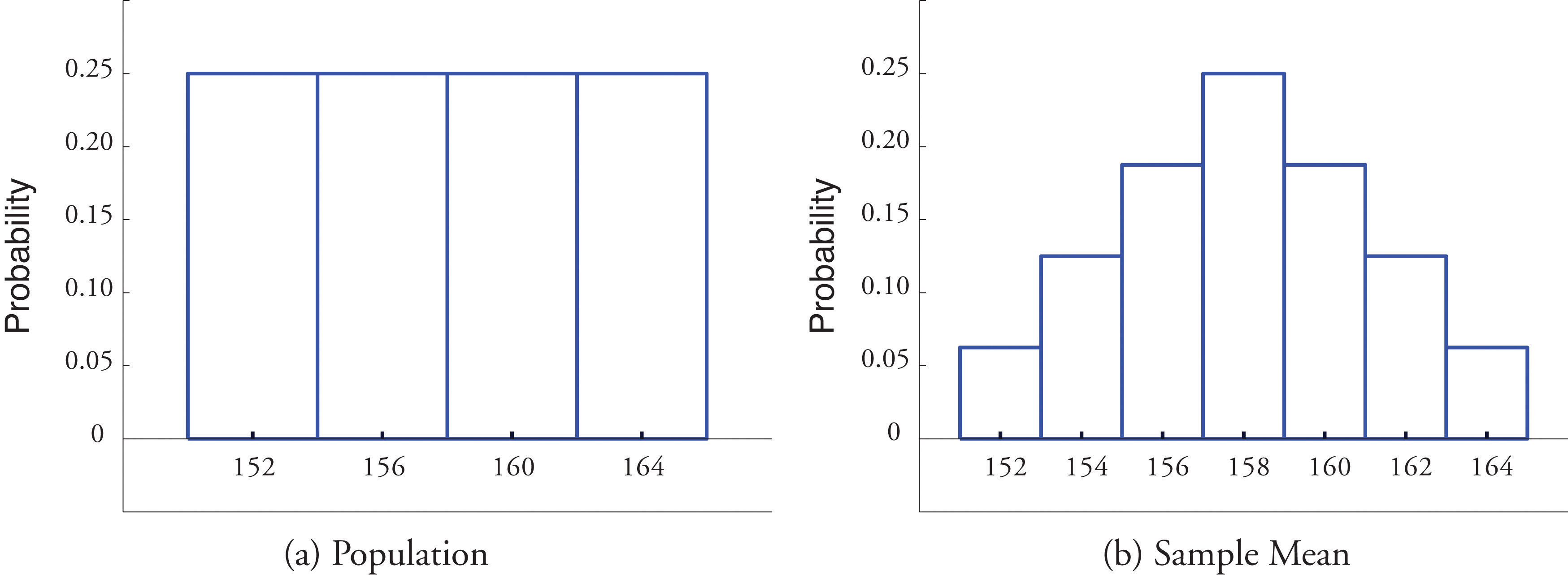
Figure 6.1 "Distribution of a Population and a Sample Mean" shows a side-by-side comparison of a histogram for the original population and a histogram for this distribution. Whereas the distribution of the population is uniform, the sampling distribution of the mean has a shape budgeted the shape of the familiar bong curve. This phenomenon of the sampling distribution of the mean taking on a bong shape even though the population distribution is not bell-shaped happens in full general. Hither is a somewhat more realistic example.

Effigy 6.1 Distribution of a Population and a Sample Mean

Suppose we have samples of size 1, 5, ten, or 20 from a population that consists entirely of the numbers 0 and 1, one-half the population 0, half 1, and so that the population mean is 0.v. The sampling distributions are:

north = 1:

$$\begin{array}{ccc}\stackrel{-}{\mathit{x}}\hfill & 0& 1\\ P\left(\stackrel{-}{\mathit{x}}\right)\hfill & 0.5& 0.5\end{array}$$

n = 5:

$$\begin{array}{ccccccc}\stackrel{-}{\mathit{x}}\hfill & 0& \mathrm{0.two}& \mathrm{0.iv}& 0.6& 0.8& 1\\ P\left(\stackrel{-}{\mathit{x}}\right)\hfill & 0.03& 0.16& 0.31& 0.31& 0.16& 0.03\end{array}$$

due north = x:

$$\begin{array}{cccccccccccc}\stackrel{-}{\mathit{x}}\hfill & 0& \mathrm{0.i}& \mathrm{0.two}& 0.3& \mathrm{0.four}& 0.5& 0.6& 0.7& \mathrm{0.eight}& \mathrm{0.nine}& 1\\ P\left(\stackrel{-}{\mathit{ten}}\right)\hfill & 0.00& 0.01& 0.04& 0.12& 0.21& 0.25& 0.21& 0.12& 0.04& 0.01& 0.00\end{array}$$

north = 20:

$$\begin{array}{cccccccccccc}\stackrel{-}{\mathit{10}}\hfill & 0& 0.05& \mathrm{0.x}& 0.15& \mathrm{0.xx}& 0.25& 0.30& 0.35& 0.40& 0.45& 0.50\\ P\left(\stackrel{-}{\mathit{10}}\right)\hfill & 0.00& 0.00& 0.00& 0.00& 0.00& 0.01& 0.04& 0.07& 0.12& 0.16& \mathrm{0.eighteen}\end{array}$$ $$\begin{array}{ccccccccccc}\stackrel{-}{\mathit{x}}\hfill & 0.55& 0.60& 0.65& 0.70& 0.75& 0.80& 0.85& 0.90& 0.95& \mathrm{i}\\ P\left(\stackrel{-}{\mathit{x}}\right)\hfill & \mathrm{0.sixteen}& 0.12& 0.07& 0.04& 0.01& 0.00& 0.00& 0.00& 0.00& 0.00\end{array}$$

Histograms illustrating these distributions are shown in Figure 6.2 "Distributions of the Sample Mean".

Effigy vi.two Distributions of the Sample Mean

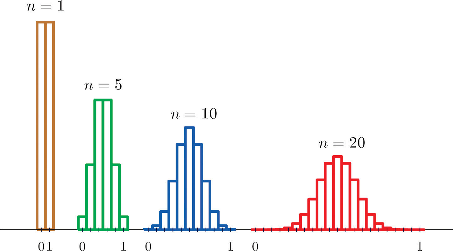
Every bit n increases the sampling distribution of $\stackrel{-}{\mathit{X}}$ evolves in an interesting way: the probabilities on the lower and the upper ends compress and the probabilities in the middle become larger in relation to them. If we were to keep to increase n so the shape of the sampling distribution would get smoother and more bell-shaped.

What we are seeing in these examples does non depend on the particular population distributions involved. In general, one may first with any distribution and the sampling distribution of the sample hateful will increasingly resemble the bell-shaped normal bend every bit the sample size increases. This is the content of the Central Limit Theorem.

The Primal Limit Theorem

For samples of size 30 or more, the sample mean is approximately unremarkably distributed, with hateful ${\mathit{\mu }}_{\stackrel{-}{\mathit{X}}}=\mathit{\mu }$ and standard deviation ${\mathit{\sigma }}_{\stackrel{-}{\mathit{X}}}=\mathit{\sigma }/\sqrt{n}$ , where n is the sample size. The larger the sample size, the meliorate the approximation.

The Cardinal Limit Theorem is illustrated for several common population distributions in Figure 6.three "Distribution of Populations and Sample Means".

Figure 6.3 Distribution of Populations and Sample Means

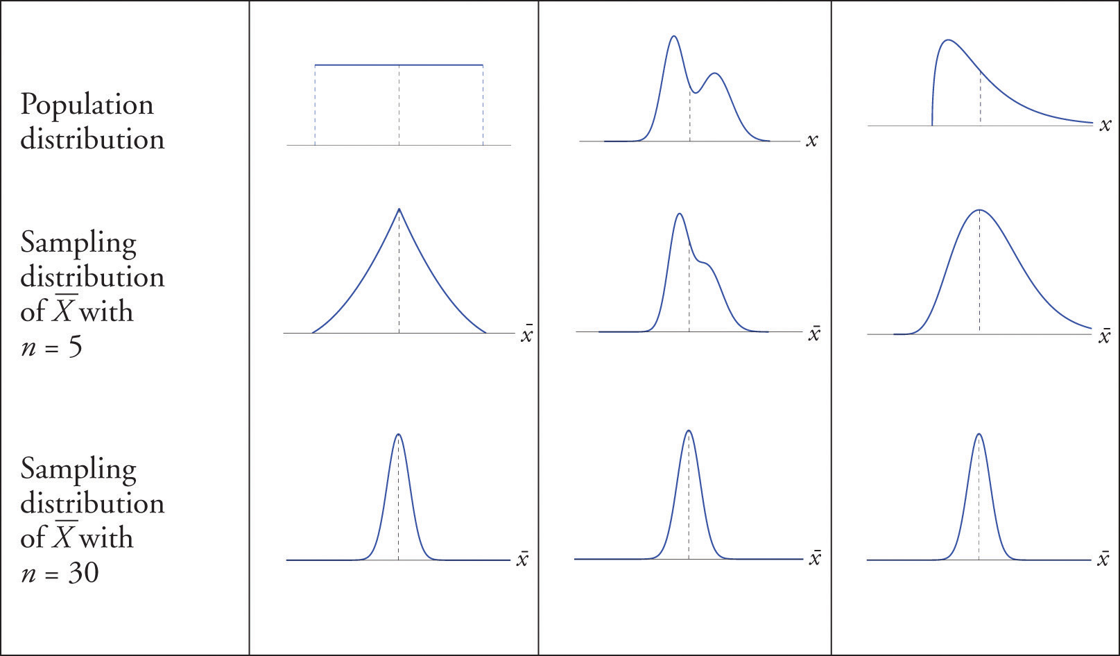
The dashed vertical lines in the figures locate the population hateful. Regardless of the distribution of the population, as the sample size is increased the shape of the sampling distribution of the sample mean becomes increasingly bong-shaped, centered on the population mean. Typically by the time the sample size is 30 the distribution of the sample hateful is practically the same as a normal distribution.

The importance of the Central Limit Theorem is that information technology allows us to make probability statements about the sample mean, specifically in relation to its value in comparison to the population mean, as nosotros will see in the examples. But to apply the result properly we must commencement realize that there are two divide random variables (and therefore ii probability distributions) at play:

1. X, the measurement of a unmarried element selected at random from the population; the distribution of X is the distribution of the population, with mean the population mean μ and standard difference the population standard deviation σ;
2. $\stackrel{-}{\mathit{Ten}}$ , the mean of the measurements in a sample of size n; the distribution of $\stackrel{-}{\mathit{X}}$ is its sampling distribution, with mean ${\mathit{\mu }}_{\stackrel{-}{\mathit{X}}}=\mathit{\mu }$ and standard difference ${\mathit{\sigma }}_{\stackrel{-}{\mathit{Ten}}}=\mathit{\sigma }/\sqrt{n}.$

Example 3

Permit $\stackrel{-}{\mathit{10}}$ be the mean of a random sample of size l drawn from a population with mean 112 and standard deviation xl.

1. Find the mean and standard difference of $\stackrel{-}{\mathit{X}}.$
2. Notice the probability that $\stackrel{-}{\mathit{X}}$ assumes a value between 110 and 114.
3. Observe the probability that $\stackrel{-}{\mathit{10}}$ assumes a value greater than 113.

Solution

1. By the formulas in the previous section

   $${\mathit{\mu }}_{\stackrel{-}{\mathit{10}}}=\mathit{\mu }=112\text{and}{\mathit{\sigma }}_{\stackrel{-}{\mathit{10}}}=\frac{\mathit{\sigma }}{\sqrt{n}}=\frac{\mathrm{forty}}{\sqrt{\mathrm{l}}}=5.65685$$

2. Since the sample size is at least 30, the Central Limit Theorem applies: $\stackrel{-}{\mathit{X}}$ is approximately commonly distributed. We compute probabilities using Effigy 12.ii "Cumulative Normal Probability" in the usual way, just existence conscientious to use ${\mathit{\sigma }}_{\stackrel{-}{\mathit{X}}}$ and non σ when we standardize:

   $$\begin{array}{ll}P(110<\stackrel{-}{\mathit{X}}<114)\hfill & =P\left(\frac{110-{\mathit{\mu }}_{\stackrel{-}{\mathit{X}}}}{{\mathit{\sigma }}_{\stackrel{-}{\mathit{X}}}}<Z<\frac{114-{\mathit{\mu }}_{\stackrel{-}{\mathit{10}}}}{{\mathit{\sigma }}_{\stackrel{-}{\mathit{X}}}}\right)\hfill \\ \hfill & =P\left(\frac{110-112}{\mathrm{v.65685}}<Z<\frac{114-112}{5.65685}\right)\hfill \\ \hfill & =P\left(\text{−}0.35<Z<0.35\right)=0.6368-0.3632=0.2736\hfill \end{array}$$

3. Similarly

   $$\begin{array}{ll}P(\stackrel{-}{\mathit{X}}>113)\hfill & =P\left(Z>\frac{113-{\mathit{\mu }}_{\stackrel{-}{\mathit{Ten}}}}{{\mathit{\sigma }}_{\stackrel{-}{\mathit{X}}}}\right)\hfill \\ \hfill & =P\left(Z>\frac{113-112}{\mathrm{five.65685}}\right)\hfill \\ \hfill & =P\left(Z>0.18\right)\hfill \\ \hfill & =\mathrm{i}-P(Z<0.18)=\mathrm{ane}-0.5714=0.4286\hfill \end{array}$$

Note that if in Note 6.11 "Case iii" nosotros had been asked to compute the probability that the value of a single randomly selected element of the population exceeds 113, that is, to compute the number P(10 > 113), we would not have been able to do so, since nosotros practise not know the distribution of X, but only that its mean is 112 and its standard deviation is xl. By contrast we could compute $P\left(\stackrel{-}{\mathit{10}}>113\right)$ fifty-fifty without complete knowledge of the distribution of 10 because the Central Limit Theorem guarantees that $\stackrel{-}{\mathit{X}}$ is approximately normal.

Example 4

The numerical population of grade betoken averages at a college has mean two.61 and standard deviation 0.five. If a random sample of size 100 is taken from the population, what is the probability that the sample mean will be between 2.51 and 2.71?

Solution

The sample mean $\stackrel{-}{\mathit{X}}$ has hateful ${\mathit{\mu }}_{\stackrel{-}{\mathit{X}}}=\mathit{\mu }=2.61$ and standard departure ${\mathit{\sigma }}_{\stackrel{-}{\mathit{10}}}=\mathit{\sigma }/\sqrt{n}=0.5/\mathrm{x}=0.05$ , so

$$\begin{array}{ll}P(\mathrm{two.51}<\stackrel{-}{\mathit{X}}<2.71)\hfill & =P\left(\frac{2.51-{\mathit{\mu }}_{\stackrel{-}{\mathit{Ten}}}}{{\mathit{\sigma }}_{\stackrel{-}{\mathit{X}}}}<Z<\frac{2.71-{\mathit{\mu }}_{\stackrel{-}{\mathit{X}}}}{{\mathit{\sigma }}_{\stackrel{-}{\mathit{X}}}}\right)\hfill \\ \hfill & =P\left(\frac{2.51-2.61}{0.05}<Z<\frac{2.71-2.61}{0.05}\right)\hfill \\ \hfill & =P\left(\text{−}\mathrm{ii}<Z<2\right)\hfill \\ \hfill & =P\left(Z<\mathrm{two}\right)-P\left(Z<\text{−}2\right)\hfill \\ \hfill & =0.9772-0.0228=0.9544\hfill \end{array}$$

Normally Distributed Populations

The Central Limit Theorem says that no matter what the distribution of the population is, as long as the sample is "large," meaning of size thirty or more, the sample mean is approximately ordinarily distributed. If the population is normal to begin with and so the sample mean likewise has a normal distribution, regardless of the sample size.

For samples of whatever size drawn from a normally distributed population, the sample mean is normally distributed, with mean ${\mathit{\mu }}_{\stackrel{-}{\mathit{10}}}=\mathit{\mu }$ and standard difference ${\mathit{\sigma }}_{\stackrel{-}{\mathit{X}}}=\mathit{\sigma }/\sqrt{\mathrm{due\; north}}$ , where due north is the sample size.

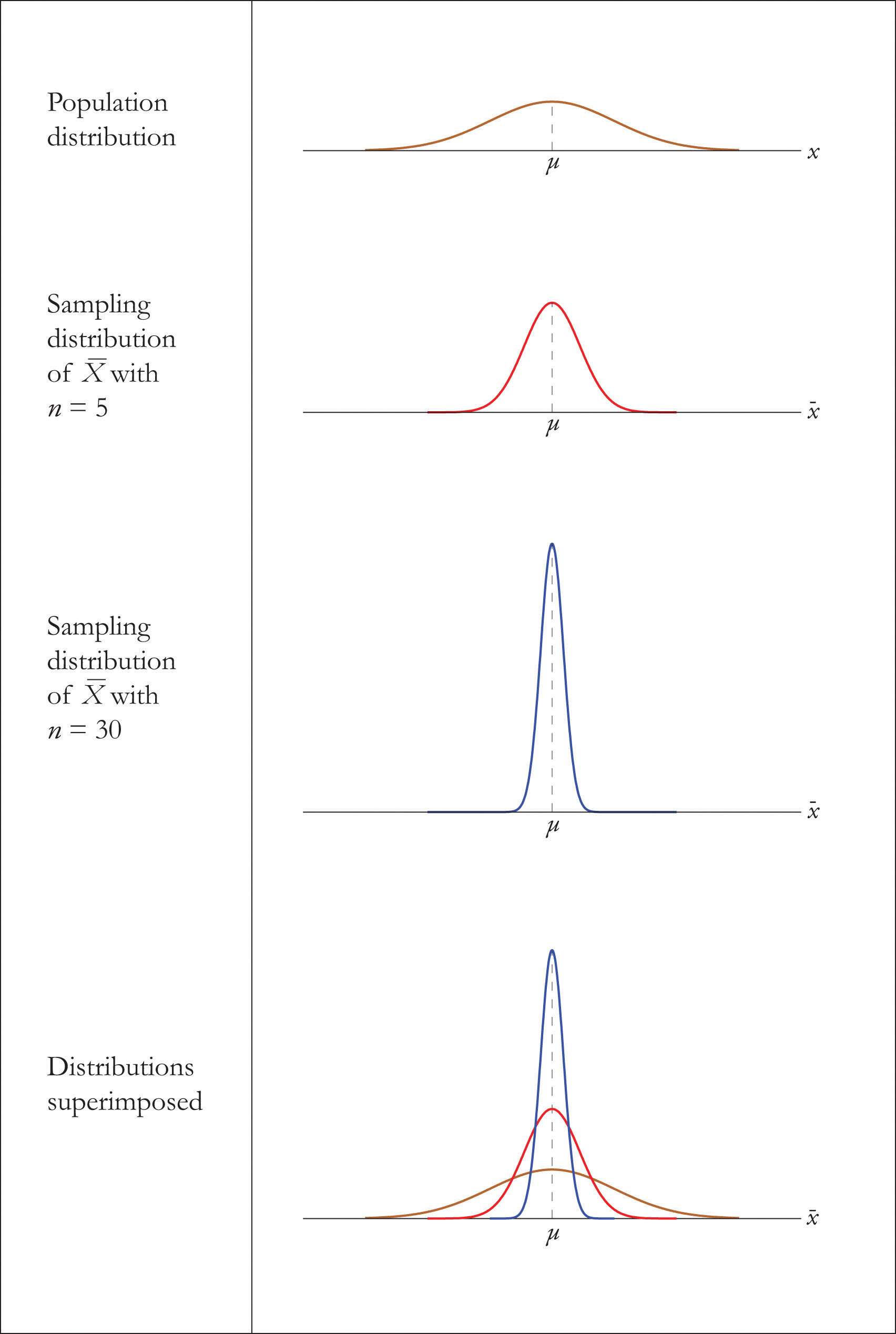
The effect of increasing the sample size is shown in Figure vi.iv "Distribution of Sample Means for a Normal Population".

Figure 6.4 Distribution of Sample Means for a Normal Population

Example 5

A prototype automotive tire has a pattern life of 38,500 miles with a standard divergence of two,500 miles. Five such tires are manufactured and tested. On the assumption that the bodily population mean is 38,500 miles and the bodily population standard deviation is 2,500 miles, discover the probability that the sample mean will exist less than 36,000 miles. Assume that the distribution of lifetimes of such tires is normal.

Solution

For simplicity we use units of thousands of miles. Then the sample mean $\stackrel{-}{\mathit{X}}$ has mean ${\mathit{\mu }}_{\stackrel{-}{\mathit{X}}}=\mathit{\mu }=38.5$ and standard difference ${\mathit{\sigma }}_{\stackrel{-}{\mathit{Ten}}}=\mathit{\sigma }/\sqrt{\mathrm{due\; north}}=\mathrm{ii.5}/\sqrt{5}=1.11803.$ Since the population is ordinarily distributed, then is $\stackrel{-}{\mathit{X}}$ , hence

$$\begin{array}{ll}P(\stackrel{-}{\mathit{Ten}}<36)\hfill & =P\left(Z<\frac{36-{\mathit{\mu }}_{\stackrel{-}{\mathit{Ten}}}}{{\mathit{\sigma }}_{\stackrel{-}{\mathit{X}}}}\right)\hfill \\ \hfill & =P\left(Z<\frac{36-38.5}{\mathrm{i.11803}}\right)\hfill \\ \hfill & =P\left(Z<\text{−}2.24\right)=0.0125\hfill \end{array}$$

That is, if the tires perform every bit designed, there is only about a one.25% chance that the boilerplate of a sample of this size would be so depression.

Example vi

An automobile battery manufacturer claims that its midgrade battery has a mean life of l months with a standard deviation of vi months. Suppose the distribution of battery lives of this particular brand is approximately normal.

1. On the assumption that the manufacturer'south claims are true, observe the probability that a randomly selected battery of this type will concluding less than 48 months.
2. On the same supposition, discover the probability that the mean of a random sample of 36 such batteries will be less than 48 months.

Solution

1. Since the population is known to have a normal distribution

   $$\begin{array}{ll}P\left(X<48\right)\hfill & =P\left(Z<\frac{48-\mathit{\mu }}{\mathit{\sigma }}\right)=P\left(Z<\frac{48-50}{\mathrm{half\; dozen}}\right)\hfill \\ \hfill & =P\left(Z<\text{−}0.33\right)=0.3707\hfill \end{array}$$

2. The sample mean has mean ${\mathit{\mu }}_{\stackrel{-}{\mathit{X}}}=\mathit{\mu }=\mathrm{l}$ and standard deviation ${\mathit{\sigma }}_{\stackrel{-}{\mathit{10}}}=\mathit{\sigma }/\sqrt{n}=\mathrm{half-dozen}/\sqrt{36}=1.$ Thus

   $$\begin{array}{ll}P\left(\stackrel{-}{\mathit{10}}<48\right)\hfill & =P\left(Z<\frac{48-{\mathit{\mu }}_{\stackrel{-}{\mathit{X}}}}{{\mathit{\sigma }}_{\stackrel{-}{\mathit{X}}}}\right)\hfill \\ \hfill & =P\left(Z<\frac{48-\mathrm{l}}{1}\right)\hfill \\ \hfill & =P\left(Z<\text{−}2\right)=0.0228\hfill \end{array}$$

Key Takeaways

• When the sample size is at to the lowest degree 30 the sample mean is normally distributed.
• When the population is normal the sample hateful is normally distributed regardless of the sample size.

Exercises

Basic

1. A population has mean 128 and standard deviation 22.

   1. Discover the hateful and standard departure of $\stackrel{-}{\mathit{Ten}}$ for samples of size 36.
   2. Find the probability that the mean of a sample of size 36 volition be within 10 units of the population mean, that is, between 118 and 138.

2. A population has mean one,542 and standard deviation 246.

   1. Find the hateful and standard deviation of $\stackrel{-}{\mathit{X}}$ for samples of size 100.
   2. Find the probability that the mean of a sample of size 100 volition be within 100 units of the population mean, that is, between 1,442 and 1,642.

3. A population has mean 73.5 and standard difference ii.5.

   1. Find the mean and standard deviation of $\stackrel{-}{\mathit{X}}$ for samples of size xxx.
   2. Observe the probability that the hateful of a sample of size 30 volition exist less than 72.

4. A population has mean 48.4 and standard divergence vi.iii.

   1. Find the mean and standard divergence of $\stackrel{-}{\mathit{X}}$ for samples of size 64.
   2. Find the probability that the hateful of a sample of size 64 volition be less than 46.seven.

5. A normally distributed population has hateful 25.6 and standard deviation three.3.

   1. Detect the probability that a unmarried randomly selected element Ten of the population exceeds 30.
   2. Find the mean and standard deviation of $\stackrel{-}{\mathit{X}}$ for samples of size 9.
   3. Detect the probability that the mean of a sample of size nine fatigued from this population exceeds 30.

6. A normally distributed population has mean 57.vii and standard divergence 12.1.

   1. Observe the probability that a single randomly selected chemical element X of the population is less than 45.
   2. Notice the mean and standard deviation of $\stackrel{-}{\mathit{X}}$ for samples of size sixteen.
   3. Find the probability that the mean of a sample of size 16 drawn from this population is less than 45.

7. A population has hateful 557 and standard difference 35.

   1. Find the mean and standard divergence of $\stackrel{-}{\mathit{X}}$ for samples of size fifty.
   2. Find the probability that the hateful of a sample of size l will exist more than 570.

8. A population has mean 16 and standard divergence 1.7.

   1. Notice the mean and standard deviation of $\stackrel{-}{\mathit{X}}$ for samples of size eighty.
   2. Find the probability that the mean of a sample of size lxxx volition be more than 16.four.

9. A normally distributed population has hateful 1,214 and standard deviation 122.

   1. Observe the probability that a single randomly selected element X of the population is betwixt i,100 and i,300.
   2. Detect the hateful and standard difference of $\stackrel{-}{\mathit{Ten}}$ for samples of size 25.
   3. Find the probability that the mean of a sample of size 25 drawn from this population is between 1,100 and 1,300.

10. A unremarkably distributed population has mean 57,800 and standard departure 750.

    1. Notice the probability that a single randomly selected element X of the population is betwixt 57,000 and 58,000.
    2. Find the mean and standard deviation of $\stackrel{-}{\mathit{Ten}}$ for samples of size 100.
    3. Find the probability that the mean of a sample of size 100 drawn from this population is between 57,000 and 58,000.

11. A population has mean 72 and standard deviation 6.

    1. Observe the mean and standard deviation of $\stackrel{-}{\mathit{X}}$ for samples of size 45.
    2. Notice the probability that the mean of a sample of size 45 volition differ from the population mean 72 past at least 2 units, that is, is either less than 70 or more than 74. (Hint: One way to solve the problem is to outset find the probability of the complementary consequence.)

12. A population has mean 12 and standard deviation ane.5.

    1. Find the mean and standard deviation of $\stackrel{-}{\mathit{Ten}}$ for samples of size 90.
    2. Find the probability that the mean of a sample of size 90 volition differ from the population mean 12 by at least 0.3 unit, that is, is either less than 11.vii or more than 12.3. (Hint: One mode to solve the trouble is to starting time observe the probability of the complementary upshot.)

Applications

13. Suppose the mean number of days to germination of a variety of seed is 22, with standard difference 2.3 days. Find the probability that the mean germination time of a sample of 160 seeds volition be within 0.5 24-hour interval of the population mean.

14. Suppose the mean length of time that a caller is placed on agree when telephoning a customer service center is 23.viii seconds, with standard departure 4.6 seconds. Observe the probability that the hateful length of time on hold in a sample of 1,200 calls volition be within 0.five second of the population hateful.

15. Suppose the hateful amount of cholesterol in eggs labeled "large" is 186 milligrams, with standard deviation 7 milligrams. Notice the probability that the hateful amount of cholesterol in a sample of 144 eggs will be within ii milligrams of the population mean.

16. Suppose that in ane region of the state the mean amount of credit carte du jour debt per household in households having credit carte du jour debt is $15,250, with standard departure $7,125. Find the probability that the mean amount of credit carte du jour debt in a sample of one,600 such households will be inside $300 of the population mean.

17. Suppose speeds of vehicles on a item stretch of roadway are unremarkably distributed with mean 36.6 mph and standard deviation one.7 mph.

    1. Find the probability that the speed X of a randomly selected vehicle is between 35 and 40 mph.
    2. Notice the probability that the mean speed $\stackrel{-}{\mathit{Ten}}$ of 20 randomly selected vehicles is between 35 and 40 mph.

18. Many sharks enter a state of tonic immobility when inverted. Suppose that in a particular species of sharks the time a shark remains in a state of tonic immobility when inverted is normally distributed with hateful 11.2 minutes and standard divergence 1.i minutes.

    1. If a biologist induces a state of tonic immobility in such a shark in order to study information technology, find the probability that the shark will remain in this land for betwixt 10 and thirteen minutes.
    2. When a biologist wishes to gauge the mean fourth dimension that such sharks stay immobile past inducing tonic immobility in each of a sample of 12 sharks, find the probability that mean fourth dimension of immobility in the sample will exist between ten and 13 minutes.

19. Suppose the mean cost across the country of a 30-day supply of a generic drug is $46.58, with standard deviation $4.84. Find the probability that the mean of a sample of 100 prices of xxx-twenty-four hours supplies of this drug will be betwixt $45 and $50.

20. Suppose the hateful length of fourth dimension between submission of a state taxation return requesting a refund and the issuance of the refund is 47 days, with standard departure 6 days. Observe the probability that in a sample of 50 returns requesting a refund, the mean such time will be more than than fifty days.

21. Scores on a mutual final exam in a large enrollment, multiple-section freshman grade are commonly distributed with mean 72.seven and standard deviation xiii.1.

    1. Find the probability that the score X on a randomly selected test paper is between 70 and fourscore.
    2. Find the probability that the mean score $\stackrel{-}{\mathit{Ten}}$ of 38 randomly selected test papers is between lxx and 80.

22. Suppose the mean weight of school children's bookbags is 17.4 pounds, with standard difference 2.2 pounds. Discover the probability that the mean weight of a sample of 30 bookbags will exceed 17 pounds.

23. Suppose that in a sure region of the land the hateful duration of outset marriages that end in divorce is 7.viii years, standard divergence 1.2 years. Observe the probability that in a sample of 75 divorces, the mean age of the marriages is at most 8 years.

24. Borachio eats at the same fast food restaurant every day. Suppose the time Ten betwixt the moment Borachio enters the eating place and the moment he is served his food is normally distributed with mean four.2 minutes and standard deviation ane.three minutes.

    1. Find the probability that when he enters the restaurant today it will be at to the lowest degree v minutes until he is served.
    2. Notice the probability that average time until he is served in eight randomly selected visits to the restaurant will exist at least five minutes.

Additional Exercises

25. A high-speed packing machine can be set to deliver between eleven and 13 ounces of a liquid. For any delivery setting in this range the amount delivered is usually distributed with mean some amount μ and with standard deviation 0.08 ounce. To calibrate the machine information technology is set to deliver a particular amount, many containers are filled, and 25 containers are randomly selected and the amount they contain is measured. Find the probability that the sample mean volition be within 0.05 ounce of the bodily mean amount being delivered to all containers.

26. A tire manufacturer states that a certain type of tire has a mean lifetime of sixty,000 miles. Suppose lifetimes are normally distributed with standard deviation $\mathit{\sigma }=\text{iii,500}$ miles.

    1. Find the probability that if you buy one such tire, it volition last only 57,000 or fewer miles. If yous had this experience, is it particularly strong evidence that the tire is not every bit good as claimed?
    2. A consumer group buys five such tires and tests them. Notice the probability that average lifetime of the five tires will be 57,000 miles or less. If the mean is so depression, is that particularly strong prove that the tire is not equally practiced as claimed?

Answers

1. 1. ${\mathit{\mu }}_{\stackrel{-}{\mathit{X}}}=128$ , ${\mathit{\sigma }}_{\stackrel{-}{\mathit{X}}}=\mathrm{iii.67}$
   2. 0.9936
3. 1. ${\mathit{\mu }}_{\stackrel{-}{\mathit{X}}}=\mathrm{73.five}$ , ${\mathit{\sigma }}_{\stackrel{-}{\mathit{X}}}=0.456$
   2. 0.0005
5. 1. 0.0918
   2. ${\mathit{\mu }}_{\stackrel{-}{\mathit{Ten}}}=25.6$ , ${\mathit{\sigma }}_{\stackrel{-}{\mathit{X}}}=1.1$
   3. 0.0000
7. 1. ${\mathit{\mu }}_{\stackrel{-}{\mathit{X}}}=557$ , ${\mathit{\sigma }}_{\stackrel{-}{\mathit{X}}}=4.9497$
   2. 0.0043
9. 1. 0.5818
   2. ${\mathit{\mu }}_{\stackrel{-}{\mathit{X}}}=1214$ , ${\mathit{\sigma }}_{\stackrel{-}{\mathit{X}}}=24.4$
   3. 0.9998
11. 1. ${\mathit{\mu }}_{\stackrel{-}{\mathit{X}}}=72$ , ${\mathit{\sigma }}_{\stackrel{-}{\mathit{Ten}}}=0.8944$
    2. 0.0250

13. 0.9940

15. 0.9994

17. 1. 0.8036
    2. one.0000

19. 0.9994

21. 1. 0.2955
    2. 0.8977

23. 0.9251

25. 0.9982

six.3 The Sample Proportion

Learning Objectives

1. To recognize that the sample proportion $\widehat{P}$ is a random variable.
2. To understand the significant of the formulas for the mean and standard deviation of the sample proportion.
3. To learn what the sampling distribution of $\widehat{P}$ is when the sample size is large.

Often sampling is done in club to estimate the proportion of a population that has a specific characteristic, such equally the proportion of all items coming off an assembly line that are defective or the proportion of all people entering a retail store who make a purchase before leaving. The population proportion is denoted p and the sample proportion is denoted $\widehat{p}.$ Thus if in reality 43% of people entering a store make a buy before leaving, p = 0.43; if in a sample of 200 people entering the shop, 78 brand a purchase, $\widehat{p}=78/200=0.39.$

The sample proportion is a random variable: it varies from sample to sample in a style that cannot be predicted with certainty. Viewed as a random variable information technology will exist written $\widehat{P}.$ It has a meanThe number about which proportions computed from samples of the same size center. ${\mathit{\mu }}_{\widehat{P}}$ and a standard departureA measure of the variability of proportions computed from samples of the aforementioned size. ${\mathit{\sigma }}_{\widehat{P}}.$ Here are formulas for their values.

Suppose random samples of size northward are drawn from a population in which the proportion with a characteristic of interest is p. The mean ${\mathit{\mu }}_{\widehat{P}}$ and standard deviation ${\mathit{\sigma }}_{\widehat{P}}$ of the sample proportion $\widehat{P}$ satisfy

$${\mathit{\mu }}_{\widehat{P}}=p\text{and}{\mathit{\sigma }}_{\widehat{P}}=\sqrt{\frac{pq}{\mathrm{due\; north}}}$$

where $q=1-p.$

The Central Limit Theorem has an analogue for the population proportion $\widehat{P}.$ To encounter how, imagine that every element of the population that has the feature of interest is labeled with a 1, and that every element that does not is labeled with a 0. This gives a numerical population consisting entirely of zeros and ones. Clearly the proportion of the population with the special characteristic is the proportion of the numerical population that are ones; in symbols,

$$p=\frac{\text{number}\text{of}1\text{s}}{\mathrm{Northward}}$$

Only of course the sum of all the zeros and ones is merely the number of ones, so the hateful μ of the numerical population is

$$\mathit{\mu }=\frac{{\displaystyle \mathrm{\Sigma }x}}{\mathrm{Due\; north}}=\frac{\text{number}\text{of}1\text{s}}{N}$$

Thus the population proportion p is the same every bit the mean μ of the respective population of zeros and ones. In the same way the sample proportion $\widehat{p}$ is the aforementioned equally the sample mean $\stackrel{-}{\mathit{x}}.$ Thus the Central Limit Theorem applies to $\widehat{P}.$ However, the condition that the sample be big is a little more complicated than merely being of size at least xxx.

The Sampling Distribution of the Sample Proportion

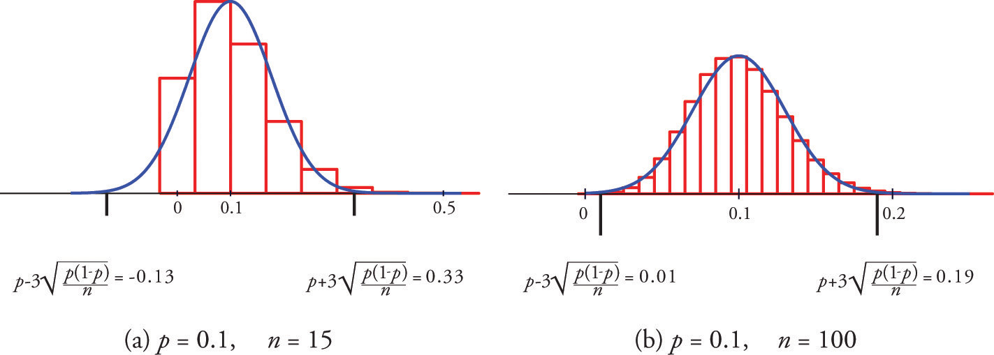
For large samples, the sample proportion is approximately normally distributed, with mean ${\mathit{\mu }}_{\widehat{P}}=p$ and standard departure ${\mathit{\sigma }}_{\widehat{P}}=\sqrt{pq/\mathrm{northward}}.$

A sample is large if the interval $\left[p\text{−}3{\mathit{\sigma }}_{\widehat{P}},p+3{\mathit{\sigma }}_{\widehat{P}}\right]$ lies wholly within the interval $\left[\mathrm{0,1}\right].$

In bodily practice p is not known, hence neither is ${\mathit{\sigma }}_{\widehat{P}}.$ In that case in society to check that the sample is sufficiently large we substitute the known quantity $\widehat{p}$ for p. This means checking that the interval

$$\left[\widehat{p}\text{−}3\sqrt{\frac{\widehat{p}(\mathrm{ane}-\widehat{p})}{n}},\widehat{p}+3\sqrt{\frac{\widehat{p}(\mathrm{one}-\widehat{p})}{n}}\right]$$

lies wholly inside the interval $\left[\mathrm{0,1}\right].$ This is illustrated in the examples.

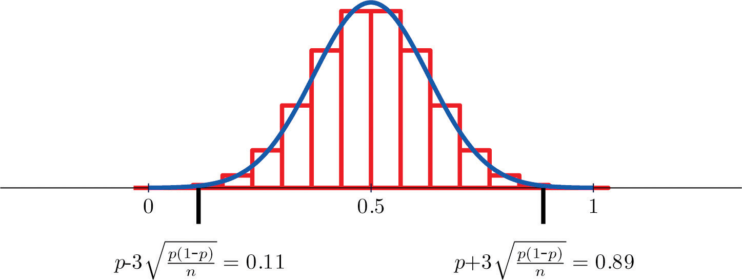
Figure six.5 "Distribution of Sample Proportions" shows that when p = 0.1 a sample of size 15 is too modest but a sample of size 100 is acceptable. Figure six.six "Distribution of Sample Proportions for " shows that when p = 0.5 a sample of size 15 is adequate.

Figure half dozen.five Distribution of Sample Proportions

Effigy half-dozen.6 Distribution of Sample Proportions for p = 0.five and n = xv

Example vii

Suppose that in a population of voters in a sure region 38% are in favor of item bond effect. Ix hundred randomly selected voters are asked if they favor the bond issue.

1. Verify that the sample proportion $\widehat{P}$ computed from samples of size 900 meets the condition that its sampling distribution be approximately normal.
2. Find the probability that the sample proportion computed from a sample of size 900 volition be within 5 percentage points of the true population proportion.

Solution

1. The information given is that p = 0.38, hence $q=1-p=0.62.$ First we use the formulas to compute the hateful and standard deviation of $\widehat{P}$ :

   $${\mathit{\mu }}_{\widehat{P}}=p=0.38\text{and}{\mathit{\sigma }}_{\widehat{P}}=\sqrt{\frac{pq}{n}}=\sqrt{\frac{\left(0.38\right)\left(0.62\right)}{900}}=0.01618$$

   So $3{\mathit{\sigma }}_{\widehat{P}}=3\left(0.01618\right)=0.04854\approx 0.05$ and so

   $$\left[p\text{−}\mathrm{three}{\mathit{\sigma }}_{\widehat{P}},p+3{\mathit{\sigma }}_{\widehat{P}}\right]=\left[0.38-0.\mathrm{05,0}.38+0.05\right]=\left[0.\mathrm{33,0}.43\right]$$

   which lies wholly within the interval $\left[\mathrm{0,1}\right]$ , so it is rubber to assume that $\widehat{P}$ is approximately usually distributed.

2. To be inside v percentage points of the true population proportion 0.38 means to be betwixt $0.38-0.05=0.33$ and $0.38+0.05=0.43.$ Thus

   $$\begin{array}{ll}P(0.33<\widehat{P}<0.43)\hfill & =P\left(\frac{0.33-{\mathit{\mu }}_{\widehat{P}}}{{\mathit{\sigma }}_{\widehat{P}}}<Z<\frac{0.43-{\mathit{\mu }}_{\widehat{P}}}{{\mathit{\sigma }}_{\widehat{P}}}\right)\hfill \\ \hfill & =P\left(\frac{0.33-0.38}{0.01618}<Z<\frac{0.43-0.38}{0.01618}\right)\hfill \\ \hfill & =P\left(\text{−}\mathrm{three.09}<Z<\mathrm{three.09}\right)\hfill \\ \hfill & =P\left(\mathrm{three.09}\right)-P\left(\text{−}3.09\right)\hfill \\ \hfill & =0.9990-0.0010=0.9980\hfill \end{array}$$

Instance 8

An online retailer claims that ninety% of all orders are shipped within 12 hours of being received. A consumer group placed 121 orders of unlike sizes and at dissimilar times of day; 102 orders were shipped within 12 hours.

1. Compute the sample proportion of items shipped within 12 hours.
2. Confirm that the sample is large enough to assume that the sample proportion is normally distributed. Use p = 0.ninety, corresponding to the assumption that the retailer's merits is valid.
3. Assuming the retailer's claim is true, find the probability that a sample of size 121 would produce a sample proportion so low every bit was observed in this sample.
4. Based on the answer to part (c), depict a conclusion about the retailer'southward merits.

Solution

1. The sample proportion is the number x of orders that are shipped inside 12 hours divided past the number n of orders in the sample:

   $$\widehat{p}=\frac{x}{\mathrm{due\; north}}=\frac{102}{121}=0.84$$

2. Since p = 0.ninety, $q=1-p=0.10$ , and n = 121,

   $${\mathit{\sigma }}_{\widehat{P}}=\sqrt{\frac{\left(0.90\right)\left(\mathrm{0.x}\right)}{121}}=0.0\stackrel{-}{27}$$

   hence

   $$\left[p\text{−}\mathrm{iii}{\mathit{\sigma }}_{\widehat{P}},p+\mathrm{iii}{\mathit{\sigma }}_{\widehat{P}}\right]=\left[\mathrm{0.xc}-0.\mathrm{08,0}.90+0.08\right]=\left[0.\mathrm{82,0}.98\right]$$

   Considering $$\left[0.82,0.98\right]\subset \left[\mathrm{0,1}\right],$$ it is appropriate to apply the normal distribution to compute probabilities related to the sample proportion $\widehat{P}.$

3. Using the value of $\widehat{P}$ from role (a) and the computation in function (b),

   $$\begin{array}{ll}P(\widehat{P}\le 0.84)\hfill & =P\left(Z\le \frac{0.84-{\mathit{\mu }}_{\widehat{P}}}{{\mathit{\sigma }}_{\widehat{P}}}\right)\hfill \\ \hfill & =P\left(Z\le \frac{0.84-0.90}{0.0\stackrel{-}{27}}\right)\hfill \\ \hfill & =P\left(Z\le \text{−}2.20\right)=0.0139\hfill \end{array}$$
4. The computation shows that a random sample of size 121 has merely virtually a one.4% chance of producing a sample proportion every bit the ane that was observed, $\widehat{p}=0.84$ , when taken from a population in which the actual proportion is 0.90. This is and so unlikely that it is reasonable to conclude that the actual value of p is less than the ninety% claimed.

Key Takeaways

• The sample proportion is a random variable $\widehat{P}.$
• There are formulas for the hateful ${\mathit{\mu }}_{\widehat{P}}$ and standard deviation ${\mathit{\sigma }}_{\widehat{P}}$ of the sample proportion.
• When the sample size is large the sample proportion is usually distributed.

Exercises

Basic

1. The proportion of a population with a characteristic of involvement is p = 0.37. Discover the mean and standard deviation of the sample proportion $\widehat{P}$ obtained from random samples of size 1,600.

2. The proportion of a population with a characteristic of interest is p = 0.82. Find the hateful and standard difference of the sample proportion $\widehat{P}$ obtained from random samples of size 900.

3. The proportion of a population with a feature of interest is p = 0.76. Discover the mean and standard departure of the sample proportion $\widehat{P}$ obtained from random samples of size i,200.

4. The proportion of a population with a characteristic of involvement is p = 0.37. Find the mean and standard departure of the sample proportion $\widehat{P}$ obtained from random samples of size 125.

5. Random samples of size 225 are drawn from a population in which the proportion with the characteristic of interest is 0.25. Decide whether or not the sample size is large enough to assume that the sample proportion $\widehat{P}$ is normally distributed.

6. Random samples of size one,600 are fatigued from a population in which the proportion with the characteristic of interest is 0.05. Determine whether or not the sample size is large enough to presume that the sample proportion $\widehat{P}$ is normally distributed.

7. Random samples of size northward produced sample proportions $\widehat{p}$ as shown. In each case decide whether or not the sample size is large enough to assume that the sample proportion $\widehat{P}$ is usually distributed.

   1. n = 50, $\widehat{p}=0.48$
   2. n = 50, $\widehat{p}=0.12$
   3. northward = 100, $\widehat{p}=0.12$

8. Samples of size northward produced sample proportions $\widehat{p}$ as shown. In each example decide whether or not the sample size is large plenty to presume that the sample proportion $\widehat{P}$ is usually distributed.

   1. northward = 30, $\widehat{p}=0.72$
   2. n = thirty, $\widehat{p}=0.84$
   3. n = 75, $\widehat{p}=0.84$

9. A random sample of size 121 is taken from a population in which the proportion with the feature of interest is p = 0.47. Find the indicated probabilities.

   1. $P\left(0.45\le \widehat{P}\le 0.50\right)$
   2. $P\left(\widehat{P}\ge 0.50\right)$

10. A random sample of size 225 is taken from a population in which the proportion with the feature of interest is p = 0.34. Find the indicated probabilities.

    1. $P\left(0.25\le \widehat{P}\le 0.40\right)$
    2. $P\left(\widehat{P}\le 0.35\right)$

11. A random sample of size 900 is taken from a population in which the proportion with the feature of interest is p = 0.62. Find the indicated probabilities.

    1. $P\left(\mathrm{0.lx}\le \widehat{P}\le 0.64\right)$
    2. $P\left(0.57\le \widehat{P}\le 0.67\right)$

12. A random sample of size 1,100 is taken from a population in which the proportion with the characteristic of interest is p = 0.28. Find the indicated probabilities.

    1. $P\left(0.27\le \widehat{P}\le 0.29\right)$
    2. $P\left(0.23\le \widehat{P}\le 0.33\right)$

Applications

13. Suppose that 8% of all males suffer some form of color blindness. Notice the probability that in a random sample of 250 men at to the lowest degree 10% volition suffer some form of color blindness. First verify that the sample is sufficiently large to use the normal distribution.

14. Suppose that 29% of all residents of a community favor annexation by a nearby municipality. Find the probability that in a random sample of 50 residents at least 35% volition favor looting. Showtime verify that the sample is sufficiently large to utilise the normal distribution.

15. Suppose that 2% of all cell phone connections by a sure provider are dropped. Find the probability that in a random sample of 1,500 calls at most forty volition be dropped. First verify that the sample is sufficiently large to use the normal distribution.

16. Suppose that in twenty% of all traffic accidents involving an injury, driver distraction in some form (for example, changing a radio station or texting) is a cistron. Find the probability that in a random sample of 275 such accidents between 15% and 25% involve driver distraction in some class. Commencement verify that the sample is sufficiently large to use the normal distribution.

17. An airline claims that 72% of all its flights to a certain region arrive on time. In a random sample of 30 contempo arrivals, 19 were on time. You may assume that the normal distribution applies.

    1. Compute the sample proportion.
    2. Assuming the airline'south claim is truthful, notice the probability of a sample of size 30 producing a sample proportion so low equally was observed in this sample.

18. A humane guild reports that 19% of all pet dogs were adopted from an animal shelter. Bold the truth of this exclamation, find the probability that in a random sample of 80 pet dogs, betwixt 15% and 20% were adopted from a shelter. You may assume that the normal distribution applies.

19. In one report it was found that 86% of all homes take a functional smoke detector. Suppose this proportion is valid for all homes. Find the probability that in a random sample of 600 homes, between 80% and 90% will have a functional smoke detector. Yous may assume that the normal distribution applies.

20. A country insurance commission estimates that 13% of all motorists in its state are uninsured. Suppose this proportion is valid. Find the probability that in a random sample of 50 motorists, at to the lowest degree 5 will be uninsured. You may assume that the normal distribution applies.

21. An outside financial auditor has observed that most 4% of all documents he examines contain an error of some sort. Bold this proportion to be accurate, find the probability that a random sample of 700 documents will contain at least thirty with some sort of mistake. You may assume that the normal distribution applies.

22. Suppose vii% of all households have no dwelling phone but depend completely on cell phones. Find the probability that in a random sample of 450 households, between 25 and 35 will have no home telephone. You may assume that the normal distribution applies.

Additional Exercises

23. Some countries allow individual packages of prepackaged goods to weigh less than what is stated on the package, bailiwick to certain conditions, such as the average of all packages being the stated weight or greater. Suppose that one requirement is that at most four% of all packages marked 500 grams can weigh less than 490 grams. Assuming that a product actually meets this requirement, find the probability that in a random sample of 150 such packages the proportion weighing less than 490 grams is at least 3%. Yous may assume that the normal distribution applies.

24. An economist wishes to investigate whether people are keeping cars longer now than in the past. He knows that five years ago, 38% of all rider vehicles in performance were at least ten years quondam. He commissions a study in which 325 automobiles are randomly sampled. Of them, 132 are 10 years old or older.

    1. Notice the sample proportion.
    2. Detect the probability that, when a sample of size 325 is fatigued from a population in which the truthful proportion is 0.38, the sample proportion will exist as large every bit the value you computed in part (a). You may assume that the normal distribution applies.
    3. Give an estimation of the result in part (b). Is at that place strong evidence that people are keeping their cars longer than was the case five years ago?

25. A state public health section wishes to investigate the effectiveness of a campaign against smoking. Historically 22% of all adults in the state regularly smoked cigars or cigarettes. In a survey commissioned past the public health department, 279 of 1,500 randomly selected adults stated that they smoke regularly.

    1. Notice the sample proportion.
    2. Find the probability that, when a sample of size 1,500 is drawn from a population in which the truthful proportion is 0.22, the sample proportion will be no larger than the value yous computed in part (a). Y'all may assume that the normal distribution applies.
    3. Give an interpretation of the result in part (b). How potent is the evidence that the campaign to reduce smoking has been effective?

26. In an endeavor to reduce the population of unwanted cats and dogs, a grouping of veterinarians set up a low-cost spay/neuter clinic. At the inception of the dispensary a survey of pet owners indicated that 78% of all pet dogs and cats in the community were spayed or neutered. After the low-cost clinic had been in functioning for three years, that figure had risen to 86%.

    1. What information is missing that y'all would need to compute the probability that a sample drawn from a population in which the proportion is 78% (respective to the assumption that the low-toll clinic had had no result) is every bit loftier every bit 86%?
    2. Knowing that the size of the original sample three years ago was 150 and that the size of the recent sample was 125, compute the probability mentioned in function (a). You may presume that the normal distribution applies.
    3. Give an estimation of the consequence in function (b). How strong is the evidence that the presence of the depression-cost clinic has increased the proportion of pet dogs and cats that take been spayed or neutered?

27. An ordinary dice is "off-white" or "counterbalanced" if each face has an equal adventure of landing on top when the dice is rolled. Thus the proportion of times a three is observed in a large number of tosses is expected to exist close to ane/6 or $0.1\stackrel{-}{6}.$ Suppose a die is rolled 240 times and shows 3 on top 36 times, for a sample proportion of 0.15.

    1. Observe the probability that a fair dice would produce a proportion of 0.15 or less. Y'all may assume that the normal distribution applies.
    2. Give an interpretation of the result in function (b). How stiff is the prove that the die is not fair?
    3. Suppose the sample proportion 0.fifteen came from rolling the die 2,400 times instead of only 240 times. Rework office (a) under these circumstances.
    4. Requite an interpretation of the outcome in part (c). How strong is the bear witness that the die is not off-white?

Answers

1. ${\mathit{\mu }}_{\widehat{P}}=0.37$ , ${\mathit{\sigma }}_{\widehat{P}}=0.012$

3. ${\mathit{\mu }}_{\widehat{P}}=0.76$ , ${\mathit{\sigma }}_{\widehat{P}}=0.012$

5. $p\pm \mathrm{iii}\sqrt{\frac{pq}{n}}=0.25\pm 0.087$ , yes

7. 1. $\widehat{p}\pm 3\sqrt{\frac{\widehat{p}\widehat{q}}{n}}=0.48\pm 0.21$ , yes
   2. $\widehat{p}\pm \mathrm{three}\sqrt{\frac{\widehat{p}\widehat{q}}{n}}=0.12\pm \mathrm{0.xiv}$ , no
   3. $\widehat{p}\pm 3\sqrt{\frac{\widehat{p}\widehat{q}}{n}}=0.12\pm \mathrm{0.x}$ , yeah
9. 1. 0.4154
   2. 0.2546
11. 1. 0.7850
    2. 0.9980

13. $p\pm 3\sqrt{\frac{pq}{n}}=0.08\pm 0.05$

    and

    $\left[0.\mathrm{03,0}.13\right]\subset \left[\mathrm{0,1}\right],0.1210$

15. $p\pm 3\sqrt{\frac{pq}{\mathrm{northward}}}=0.02\pm 0.01$

    and

    $\left[0.\mathrm{01,0}.03\right]\subset \left[\mathrm{0,1}\right],0.9671$

17. 1. 0.63
    2. 0.1446

19. 0.9977

21. 0.3483

23. 0.7357

25. 1. 0.186
    2. 0.0007
    3. In a population in which the truthful proportion is 22% the run a risk that a random sample of size 1500 would produce a sample proportion of 18.six% or less is merely vii/100 of ane%. This is stiff prove that currently a smaller proportion than 22% smoke.
27. 1. 0.2451
    2. We would expect a sample proportion of 0.15 or less in about 24.5% of all samples of size 240, so this is practically no evidence at all that the die is not off-white.
    3. 0.0139
    4. We would expect a sample proportion of 0.15 or less in only about 1.4% of all samples of size 2400, so this is strong evidence that the die is not fair.

Sampling And Normal Distribution Answers,

Source: https://saylordotorg.github.io/text_introductory-statistics/s10-sampling-distributions.html

Posted by: smithhower1967.blogspot.com

Share this post